Limits at infinity are an important concept in calculus that helps us understand how a function behaves when its input becomes extremely large or extremely small. Instead of examining what happens at a particular value of a variable, we study what happens as the variable increases without bound or decreases without bound. This concept allows us to describe the long-term behavior of mathematical functions, identify horizontal asymptotes, and understand how graphs behave far away from the origin.
Limits at infinity are especially useful when studying rational functions, polynomial expressions, exponential functions, and other mathematical models. They also have practical applications in physics, engineering, economics, computer science, and many other fields. In this beginner-friendly guide, we will learn what limits at infinity mean, how to calculate them, which rules are useful, and how to solve common examples step by step.
What Are Limits at Infinity?
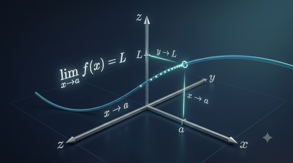
A limit at infinity describes the behavior of a function as its input variable increases or decreases without bound.
In calculus, infinity does not represent an ordinary number. Instead, it describes a process in which a variable continues to grow larger or smaller without reaching a final value.
For example, imagine a function whose output gets closer and closer to 5 as the input becomes larger. The output might never become exactly 5, but it can approach 5 as the input increases indefinitely.
This behavior can be described using a limit at infinity.
Formula (Text Block):
limₓ→∞ f(x) = L
This means that the value of the function f(x) approaches L as x approaches positive infinity.
Similarly, we can study what happens when x decreases without bound.
Formula (Text Block):
limₓ→−∞ f(x) = L
This means that f(x) approaches L as x approaches negative infinity.
The value L is a finite number that the function approaches. However, a limit at infinity does not always have to be finite. Depending on the function, its value may increase or decrease without bound, or the limit may fail to exist.
Understanding Positive and Negative Infinity
To understand limits at infinity, it is important to distinguish between positive infinity and negative infinity.
Positive Infinity
Positive infinity describes a situation in which the value of x increases without bound.
For example, x may take values such as 10, 100, 1,000, 10,000, and increasingly larger numbers.
We represent this process as:
Formula (Text Block):
x → ∞
Consider the function below.
Formula (Text Block):
f(x) = 1/x
As x becomes larger and larger, the value of 1/x becomes smaller and closer to zero.
For example:
When x = 10, f(x) = 0.1.
When x = 100, f(x) = 0.01.
When x = 1,000, f(x) = 0.001.
Therefore, the function approaches zero as x approaches positive infinity.
Formula (Text Block):
limₓ→∞ 1/x = 0
Negative Infinity
Negative infinity describes a situation in which x decreases without bound.
We represent this process as:
Formula (Text Block):
x → −∞
For the same function, f(x) = 1/x, consider increasingly negative values of x.
When x = −10, f(x) = −0.1.
When x = −100, f(x) = −0.01.
When x = −1,000, f(x) = −0.001.
The function approaches zero from the negative side.
Formula (Text Block):
limₓ→−∞ 1/x = 0
Although the function approaches zero from different directions, both limits have the same value.
Why Are Limits at Infinity Important?
Limits at infinity help us understand the overall behavior of functions rather than focusing only on individual input values.
They are useful for several reasons.
Understanding Long-Term Behavior
A function may behave differently for small inputs and large inputs. Limits at infinity help determine what happens as the input becomes extremely large.
For example, a mathematical model may predict that a particular quantity gradually approaches a fixed value. A limit can describe that long-term behavior.
Finding Horizontal Asymptotes
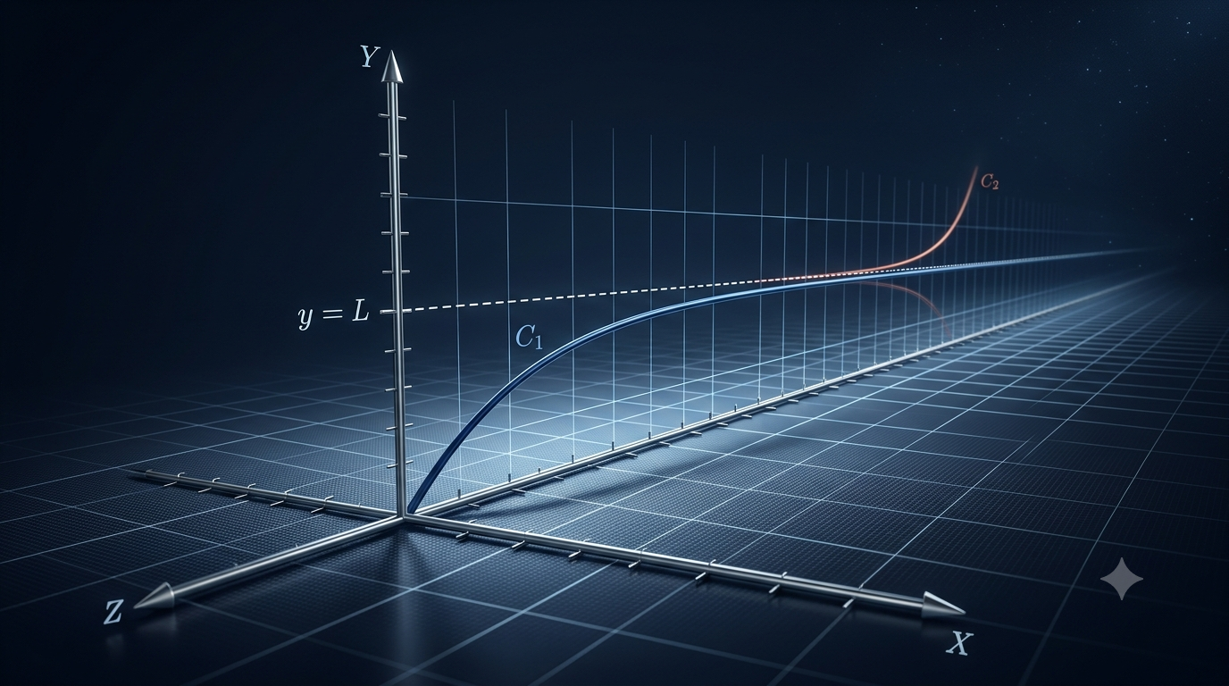
A horizontal asymptote is a horizontal line that a function approaches as x tends toward positive or negative infinity.
If the following limit exists and equals L, then y = L is a horizontal asymptote in that direction.
Formula (Text Block):
limₓ→∞ f(x) = L
For example, consider:
Formula (Text Block):
f(x) = 3 + 2/x
As x approaches infinity, 2/x approaches zero. Therefore, the function approaches 3.
Formula (Text Block):
limₓ→∞ (3 + 2/x) = 3
The graph has a horizontal asymptote at y = 3.
Analyzing Mathematical Models
Limits at infinity are also useful for examining models of population growth, production costs, energy consumption, and other quantities that change with time or input.
They help mathematicians determine whether a quantity approaches a fixed value, continues increasing, or decreases toward zero.
Basic Rules for Limits at Infinity
Several standard rules make it easier to calculate limits at infinity.
Suppose the relevant limits exist and the expressions involved are defined appropriately.
The Limit of a Constant
A constant remains unchanged regardless of how large or small x becomes.
Formula (Text Block):
limₓ→∞ c = c
For example:
Formula (Text Block):
limₓ→∞ 7 = 7
The output is always 7, so the limit is 7.
The Limit of a Reciprocal Function
For a positive integer n:
Formula (Text Block):
limₓ→∞ 1/xⁿ = 0
As x becomes larger, the denominator grows, causing the fraction to approach zero.
For example:
Formula (Text Block):
limₓ→∞ 1/x² = 0
This rule is particularly useful when simplifying rational functions.
The Sum Rule
If two functions approach finite limits A and B, the limit of their sum is A + B.
Formula (Text Block):
limₓ→∞ [f(x) + g(x)] = A + B
For example:
Formula (Text Block):
limₓ→∞ (4 + 5/x) = 4 + 0 = 4
The fraction approaches zero, while the constant remains unchanged.
The Product Rule
If two functions approach finite limits A and B, their product approaches AB.
Formula (Text Block):
limₓ→∞ [f(x) × g(x)] = A × B
For example, if one function approaches 2 and another approaches 3, their product approaches 6.
These rules simplify many problems, although additional care is needed when one or both functions become unbounded.
Limits at Infinity of Rational Functions
Rational functions are expressions written as the ratio of two polynomials. They are among the most common functions encountered when calculating limits at infinity.
A rational function has the general form:
Formula (Text Block):
f(x) = P(x)/Q(x)
Here, P(x) and Q(x) are polynomials, and Q(x) must not equal zero wherever the function is defined.
For rational functions, comparing the degrees of the numerator and denominator is often the easiest method.
The degree of a polynomial is the highest power of its variable with a nonzero coefficient.
Case 1: The Degree of the Numerator Is Smaller
Consider:
Formula (Text Block):
f(x) = 4x/(x² + 1)
The numerator has degree 1, while the denominator has degree 2.
Divide both the numerator and denominator by x², the highest power in the denominator.
Formula (Text Block):
f(x) = (4/x)/(1 + 1/x²)
As x approaches infinity, both 4/x and 1/x² approach zero.
Therefore:
Formula (Text Block):
limₓ→∞ 4x/(x² + 1) = 0
General Rule: If the numerator has a lower degree than the denominator, the limit is zero.
Case 2: The Degrees Are Equal
Consider:
Formula (Text Block):
f(x) = (5x² + 3)/(2x² − 7)
The numerator and denominator both have degree 2.
Divide every term by x².
Formula (Text Block):
f(x) = (5 + 3/x²)/(2 − 7/x²)
As x approaches infinity, the fractions 3/x² and 7/x² approach zero.
The remaining expression approaches 5/2.
Formula (Text Block):
limₓ→∞ (5x² + 3)/(2x² − 7) = 5/2
General Rule: If the numerator and denominator have the same degree, the limit equals the ratio of their leading coefficients.
The leading coefficient is the coefficient of the term with the highest power.
Case 3: The Degree of the Numerator Is Greater
Consider:
Formula (Text Block):
f(x) = (3x³ + 2)/(x² + 1)
The numerator has degree 3, while the denominator has degree 2.
For large positive values of x, the highest-degree terms dominate the behavior of the function.
The expression behaves approximately like:
Formula (Text Block):
f(x) ≈ 3x³/x² = 3x
As x approaches positive infinity, 3x increases without bound.
Therefore:
Formula (Text Block):
limₓ→∞ (3x³ + 2)/(x² + 1) = ∞
This limit is unbounded rather than a finite real number.
General Rule: If the numerator has a higher degree than the denominator, the function’s magnitude grows without bound. The direction of that growth depends on the leading terms and whether x approaches positive or negative infinity.
Limits at Infinity of Polynomial Functions
Polynomial functions are expressions involving nonnegative integer powers of a variable, combined with constants and coefficients.
Examples include:
Formula (Text Block):
f(x) = 2x² + 3x + 1
The behavior of a polynomial at infinity is primarily determined by its highest-degree term.
For example:
Formula (Text Block):
f(x) = 2x² + 3x + 1
As x approaches positive infinity, the term 2x² grows much faster than 3x or 1. Consequently, the function increases without bound.
Formula (Text Block):
limₓ→∞ (2x² + 3x + 1) = ∞
Now consider a linear function:
Formula (Text Block):
f(x) = −4x + 6
As x approaches positive infinity, the term −4x decreases without bound. The constant 6 does not change this behavior.
Formula (Text Block):
limₓ→∞ (−4x + 6) = −∞
When working with polynomial functions, examine the leading term first. Its coefficient, degree, and the direction in which x approaches infinity determine the function’s end behavior.
Limits at Infinity Involving Square Roots
Some limits at infinity contain square roots. These expressions may require simplification before their behavior becomes clear.
Consider:
Formula (Text Block):
f(x) = √(x² + 1)/x
For positive x, we can rewrite the expression as:
Formula (Text Block):
f(x) = √(1 + 1/x²)
As x approaches positive infinity, 1/x² approaches zero. Therefore:
Formula (Text Block):
limₓ→∞ √(x² + 1)/x = 1
However, the result changes when x approaches negative infinity. In that direction, x is negative, and the square root √(x²) equals |x|, not simply x.
For negative x, |x| = −x. Consequently:
Formula (Text Block):
limₓ→−∞ √(x² + 1)/x = −1
This example illustrates why absolute values and the direction of infinity matter when working with square roots.
Limits at Infinity and Horizontal Asymptotes
Horizontal asymptotes describe the horizontal lines that a graph approaches as x tends toward positive or negative infinity.
Suppose:
Formula (Text Block):
limₓ→∞ f(x) = L
If L is finite, then y = L is a horizontal asymptote on the right-hand side of the graph.
Similarly, if:
Formula (Text Block):
limₓ→−∞ f(x) = M
and M is finite, then y = M is a horizontal asymptote on the left-hand side of the graph.
The values L and M do not have to be equal.
For example, consider:
Formula (Text Block):
f(x) = x/√(x² + 1)
As x approaches positive infinity, the function approaches 1.
Formula (Text Block):
limₓ→∞ x/√(x² + 1) = 1
As x approaches negative infinity, the function approaches −1.
Formula (Text Block):
limₓ→−∞ x/√(x² + 1) = −1
Therefore, this function has two horizontal asymptotes: y = 1 and y = −1.
A function can have different horizontal asymptotes in opposite directions. It may also have no horizontal asymptote if its limits do not approach finite values.
Common Mistakes When Solving Limits at Infinity
Beginners often make a few predictable mistakes when working with limits at infinity. Understanding these errors can make calculations more accurate.
Treating Infinity as an Ordinary Number
Infinity is not a real number that can be substituted directly into a function. A limit describes the behavior of a function as its input grows without bound.
For example, it is incorrect to treat 1/∞ as an ordinary fraction. Instead, the mathematical statement is that 1/x approaches zero as x approaches positive infinity.
Ignoring the Highest-Degree Terms
When evaluating rational functions, students sometimes focus on every term equally. However, the highest-degree terms usually determine the end behavior.
For example:
Formula (Text Block):
limₓ→∞ (7x² + 4x + 1)/(3x² − 5) = 7/3
The lower-degree terms become insignificant relative to x² as x increases.
Assuming Every Limit Equals Zero
Not every function approaches zero at infinity.
For example:
Formula (Text Block):
limₓ→∞ (2x + 1) = ∞
The function increases without bound rather than approaching zero.
Ignoring Negative Infinity
The behavior of a function at positive infinity may differ from its behavior at negative infinity. This is especially important for odd powers and expressions involving square roots.
Whenever a problem includes both directions, calculate each limit separately.
Confusing an Unbounded Limit With a Finite Limit
If a function grows without bound, its limit is described as infinity or negative infinity when the corresponding behavior is established. These are not finite real-valued limits.
A limit may also fail to exist because the function oscillates or behaves differently without approaching a single value. Therefore, it is important to examine the function rather than assume a result.
Applications of Limits at Infinity
Limits at infinity are not restricted to textbook exercises. They are useful for understanding real-world behavior in several areas.
Physics and Engineering
In physics, limits can describe how a system behaves as time increases or how a quantity changes under extreme conditions. Engineers can use mathematical models to study long-term system performance, signal behavior, and theoretical operating limits.
Economics and Business
In economics, limits can help describe situations in which costs, returns, or other quantities approach a stable value as production or market activity increases.
For example, a model of average cost might approach a particular value as the number of products manufactured becomes very large.
Computer Science
Limits are useful when studying the growth of algorithms and computational complexity. They help describe how the time or memory required by an algorithm changes as the input size increases.
For example, comparing functions that grow linearly and quadratically helps explain why some algorithms become less practical for very large inputs.
Environmental and Biological Models
Mathematical models of populations, resource use, and environmental processes sometimes approach a stable level. Limits can help describe such long-term behavior, provided the assumptions of the model remain appropriate.
In each application, a limit provides a mathematical description of a model’s behavior. It does not guarantee that a real system will follow that model indefinitely.
Practice Examples
The following examples reinforce the main rules for calculating limits at infinity.
Example 1: A Simple Reciprocal
Find the limit:
Formula (Text Block):
limₓ→∞ 8/x
As x becomes larger, the denominator increases while the numerator remains constant. Therefore, the fraction approaches zero.
Answer (Text Block):
limₓ→∞ 8/x = 0
Example 2: A Rational Function With Equal Degrees
Find the limit:
Formula (Text Block):
limₓ→∞ (6x² + 4)/(3x² + 2)
Both the numerator and denominator have degree 2. Divide each term by x².
Formula (Text Block):
limₓ→∞ (6 + 4/x²)/(3 + 2/x²)
The fractional terms approach zero, leaving 6/3.
Answer (Text Block):
limₓ→∞ (6x² + 4)/(3x² + 2) = 2
Example 3: A Polynomial
Find the limit:
Formula (Text Block):
limₓ→∞ (x³ − 2x + 5)
The highest-degree term is x³. As x approaches positive infinity, x³ increases without bound, so the entire polynomial also increases without bound.
Answer (Text Block):
limₓ→∞ (x³ − 2x + 5) = ∞
Example 4: A Limit at Negative Infinity
Find the limit:
Formula (Text Block):
limₓ→−∞ 1/x²
As x becomes increasingly negative, x² becomes increasingly positive and large. Therefore, the reciprocal approaches zero.
Answer (Text Block):
limₓ→−∞ 1/x² = 0
Example 5: A Rational Function With a Lower-Degree Numerator
Find the limit:
Formula (Text Block):
limₓ→∞ (2x + 3)/(x² + 4)
The denominator has a higher degree than the numerator. The fraction therefore approaches zero.
Answer (Text Block):
limₓ→∞ (2x + 3)/(x² + 4) = 0
Practising examples involving constants, polynomials, rational functions, and negative infinity will help you recognize which rule to use in different situations.
Conclusion
Limits at infinity are a fundamental part of calculus because they explain how functions behave when their input values become extremely large or extremely negative. They help us analyze long-term trends, calculate limits of rational and polynomial functions, and identify horizontal asymptotes. The most useful starting point is to examine the highest-degree terms of a rational function and determine whether the function approaches a finite value, zero, or grows without bound. It is equally important to distinguish between positive and negative infinity, especially when expressions involve odd powers or square roots. With regular practice, limits at infinity become easier to recognize and solve. Understanding this topic also provides a strong foundation for studying continuity, derivatives, integrals, and more advanced applications of calculus.
FAQs
1. What are limits at infinity in calculus?
Limits at infinity describe how a function behaves when its input variable increases or decreases without bound. Instead of calculating the function at one specific value, we examine what happens as the variable becomes extremely large or extremely negative. For example, the function f(x) = 1/x approaches zero as x approaches positive infinity. Limits at infinity help us understand the long-term behavior of functions, identify horizontal asymptotes, and analyze mathematical models. They are important in calculus because they provide a foundation for studying function behavior, continuity, derivatives, and several advanced mathematical concepts.
2. What is the difference between a limit at infinity and infinity itself?
Infinity is a concept that represents something without an upper or lower bound, rather than an ordinary real number. A limit at infinity describes the behavior of a function as its input increases or decreases without bound. For example, limₓ→∞ 1/x = 0 means that the function approaches zero as x increases indefinitely. It does not mean that infinity is a number that can be substituted directly into the function. Understanding this distinction is important because limits describe approaching behavior, not necessarily a value that the function reaches at a particular input.
3. How do you calculate limits at infinity?
To calculate a limit at infinity, first identify the type of function and examine how its terms behave as the variable becomes extremely large. For rational functions, compare the degrees of the numerator and denominator. If the numerator has a lower degree, the limit is zero. If both degrees are equal, divide the leading coefficient of the numerator by the leading coefficient of the denominator. If the numerator has a higher degree, examine the leading terms to determine whether the function grows toward positive or negative infinity. Simplifying expressions and dividing by the highest power of the variable can make calculations easier.
4. What is the limit of 1/x as x approaches infinity?
The limit of 1/x as x approaches positive infinity is zero. As x increases, the denominator becomes larger, causing the fraction to become smaller. For example, when x equals 10, the function equals 0.1. When x equals 100, it equals 0.01. As x continues increasing, the function gets closer to zero without becoming negative. Therefore, limₓ→∞ 1/x = 0. The same function also approaches zero as x approaches negative infinity, although its values approach zero from the negative side. This example demonstrates how limits describe the long-term behavior of mathematical functions.
5. What are the three main rules for limits at infinity of rational functions?
The three main rules depend on the degrees of the numerator and denominator. First, if the numerator has a lower degree than the denominator, the limit is zero. Second, if both have the same degree, the limit equals the ratio of their leading coefficients. Third, if the numerator has a higher degree, the function’s magnitude generally grows without bound, although its direction depends on the leading terms and the direction of infinity. These rules provide a quick method for solving many rational-function problems without lengthy calculations. However, always check the signs and the direction in which the variable approaches infinity.
6. What is a horizontal asymptote in calculus?
A horizontal asymptote is a horizontal line that a function approaches as its input variable tends toward positive infinity or negative infinity. Its equation generally has the form y = L, where L is the finite value of the corresponding limit. For example, consider f(x) = 2 + 3/x. As x approaches positive infinity, 3/x approaches zero, so the function approaches 2. Therefore, y = 2 is a horizontal asymptote. A function may have different horizontal asymptotes in opposite directions, one horizontal asymptote, or none. The existence of a horizontal asymptote does not mean the graph can never cross that line.
7. Can a limit at infinity be positive or negative infinity?
Yes. A limit at infinity can describe a function that increases or decreases without bound. For example, limₓ→∞ x² = ∞ because the square of an increasingly large positive number continues increasing. In contrast, limₓ→∞ (−x²) = −∞ because the function decreases without bound. These results describe unbounded behavior rather than finite real-valued limits. It is important to examine the leading term, its coefficient, and whether the variable approaches positive or negative infinity. A function may also fail to have a limit if it oscillates indefinitely instead of approaching a single value or a consistent unbounded direction.
8. What is the difference between limits at positive infinity and negative infinity?
A limit at positive infinity examines a function as x increases without bound, while a limit at negative infinity examines its behavior as x decreases without bound. The two limits may be equal or different. For example, the function f(x) = 1/x approaches zero from the positive side as x approaches positive infinity and from the negative side as x approaches negative infinity. Both limits equal zero. However, for f(x) = x³, the function approaches positive infinity in the positive direction and negative infinity in the negative direction. Calculating both limits separately helps determine the overall shape and end behavior of a graph.
9. Why are limits at infinity important in real life?
Limits at infinity are useful for understanding the long-term behavior of mathematical models. In physics and engineering, they can describe how quantities behave as time increases or system conditions change. In economics, limits may help analyze models of average costs or returns as production grows. In computer science, studying how functions grow helps compare algorithms as input sizes become very large. Limits also appear in models of population growth and environmental processes that approach stable levels. These applications depend on the assumptions of each mathematical model. Limits provide a way to describe predicted behavior, but real-world systems do not always follow mathematical models indefinitely.
10. What mistakes should beginners avoid when solving limits at infinity?
Beginners should avoid treating infinity as an ordinary number that can be directly substituted into a function. They should also avoid assuming that every limit at infinity equals zero. Some functions approach a finite constant, while others increase or decrease without bound. Another common mistake is ignoring the highest-degree terms when evaluating rational functions. Students should also remember that positive infinity and negative infinity can produce different results, particularly for odd powers and square-root expressions. Finally, a limit that approaches infinity is not a finite real-valued limit. Practising different examples and checking the signs of the leading terms can help prevent these mistakes.